Dynamic Programming to Solve the Knapsack Problem
Dynamic Programming is a method used to solve problems by breaking them down into simpler subproblems, solving each subproblem just once, and storing their solutions – ideally in a table – to avoid redundant calculations.
Identifying whether a problem can be effectively solved
using Dynamic Programming (DP) involves recognizing certain characteristics in
the problem. Here are key indicators that suggest a problem might be a good
candidate for a DP approach:
1. Overlapping Subproblems:
- If the problem
can be broken down into smaller subproblems and these subproblems recur
multiple times in the process of solving the problem, it's a sign that DP might
be useful. In such cases, solving each subproblem once and storing its solution
to avoid redundant calculations can significantly improve efficiency.
2. Optimal Substructure:
- A problem has an
optimal substructure if an optimal solution to the problem contains optimal
solutions to its subproblems. This means that the problem can be solved by
combining optimal solutions of its smaller parts. For instance, in the shortest
path problem, the shortest path from point A to point C through B is the
combination of the shortest path from A to B and from B to C.
The concept of optimal substructure is a key characteristic
in many dynamic programming problems, including the 0/1 Knapsack Problem.
Optimal substructure means that an optimal solution to a problem can be
constructed from optimal solutions of its subproblems. Let's explore this
concept in the context of the 0/1 Knapsack Problem.
Optimal Substructure in the 0/1 Knapsack Problem:
1. Breaking Down the Problem:
- Consider the
decision for the last item in the list (say item `n` with weight `w_n` and
value `v_n`). For a knapsack of capacity `W`, you have two choices: include
item `n` or exclude it.
- The optimal
solution for the problem with `n` items and capacity `W` thus depends on the
optimal solutions for smaller problems:
- If item `n` is
excluded, the problem reduces to finding the optimal solution for `n-1` items
with capacity `W`.
- If item `n` is
included, the problem reduces to finding the optimal solution for `n-1` items
with a reduced capacity of `W - w_n`.
2. Optimal Solutions of Subproblems:
- The optimal value
for the knapsack with capacity `W` and `n` items, `Opt(n, W)`, can be expressed
in terms of the solutions to these smaller subproblems:
- If item `n` is
excluded: `Opt(n, W) = Opt(n-1, W)`
- If item `n` is
included: `Opt(n, W) = v_n + Opt(n-1, W - w_n)`
- The overall
optimal solution is the maximum of these two options:
- `Opt(n, W) =
max(Opt(n-1, W), v_n + Opt(n-1, W - w_n))`
3. Constructing the Optimal Solution:
- This relationship
shows the optimal substructure of the problem. The optimal solution for the
problem with `n` items and capacity `W` is built from the optimal solutions of
smaller problems (either including or excluding the `n`-th item).
- This structure
allows for solving the problem efficiently using dynamic programming, where the
solutions to smaller subproblems are stored and used to construct solutions to
larger problems.
Example:
For instance, if the optimal solution for a 50 kg knapsack
with 3 items includes the 3rd item, then this solution must also include the
optimal solution for a 20 kg knapsack with the first 2 items (assuming the 3rd
item weighs 30 kg).
3. Memoization or Tabulation:
- If the problem
allows for storing the results of intermediate subproblems (either through
memoization or tabulation), then DP can be an effective strategy. Memoization
is the top-down approach where you solve the problem recursively and store the
results, while tabulation is the bottom-up approach using a table to store the
results of subproblems.
4. Decision Making at Each Step:
- If the problem
involves making decisions at each step that depend on the results of smaller
subproblems, DP might be suitable. This is common in optimization problems
where each decision impacts the overall outcome.
5. A Clear Recursive Solution:
- If a problem can
be solved by a recursive algorithm but leads to exponential time complexity due
to redundant calculations, DP might be a good fit. A clear sign is if the
recursive solution has a small number of distinct states but recalculates the
same states many times.
Recursive Structure:
The recursive solution to the 0/1 Knapsack Problem involves
making a decision at each step about whether to include an item in the knapsack
or not. Let's define `knapsack(i, W)` as the maximum value that can be achieved
with the first `i` items and a knapsack of capacity `W`.
1. Base Cases:
- If `i == 0` (no
items) or `W == 0` (no capacity), the maximum value is 0.
2. Recursive Calls:
- For each item
`i`, you have two choices: include the item in the knapsack or exclude it.
- If you include
the item, you reduce the capacity of the knapsack by the weight of that item
and add the value of that item to your total.
- If you exclude
the item, you move to the next item without changing the current capacity or
value.
3. Formulating the Recursive Relation:
- The maximum value
`knapsack(i, W)` can be expressed as the maximum of two scenarios:
- Excluding the
`i`-th item: `knapsack(i-1, W)`
- Including the
`i`-th item (if it fits): `value[i] + knapsack(i-1, W - weight[i])`
4. Expressing the Recursive Formula:
- `knapsack(i, W) =
max(knapsack(i-1, W), value[i] + knapsack(i-1, W - weight[i]))` (if `weight[i]
≤ W`)
- Otherwise, if
`weight[i] > W`, you cannot include the `i`-th item, so it's just:
`knapsack(i, W) = knapsack(i-1, W)`
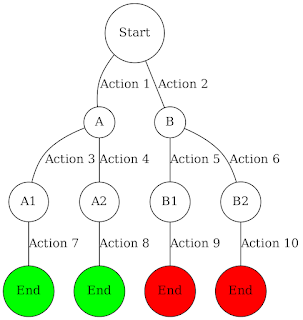
Understanding the Recursive Calls:
- At each step, you consider one item at a time, deciding
whether to include it in the optimal subset.
- The recursion explores all combinations of items,
effectively building up a decision tree where each node represents a state
(defined by the remaining capacity and the set of items considered so far).
Why This Leads to Overlapping Subproblems:
- In this recursive structure, many subproblems are solved
multiple times. For instance, `knapsack(i, W)` might be called from different
paths in the decision tree with the same values of `i` and `W`.
Transition to Dynamic Programming:
- To avoid redundant calculations in these overlapping
subproblems, Dynamic Programming stores the results of subproblems in a table.
Thus, each subproblem is solved only once, significantly reducing the
computational complexity.
This recursive understanding is crucial for implementing a
Dynamic Programming solution, as it provides the framework upon which the DP
table is built and filled out.
6. Problem Can Be Framed as a State Transition System:
- If the problem
can be represented as a series of decisions or transitions between states, and
you need to find an optimal path through the state space, DP is often
applicable. This is typical in problems involving sequences or paths (like
sequence alignment in bioinformatics or certain types of graph problems).
Key Takeaway:
When faced with a problem, analyze it for these
characteristics. If several of them apply, it's likely that Dynamic Programming
is a suitable approach. However, remember that implementing DP might still be
challenging, and understanding the underlying recursive structure of the
problem is often the first step in crafting a DP solution.
Example of the 0/1 Knapsack Problem:
- Knapsack Capacity: 50 kg
- Items:
1. Item A: Weight =
10 kg, Value = $60
2. Item B: Weight =
20 kg, Value = $100
3. Item C: Weight =
30 kg, Value = $120
Why the Solution Uses Dynamic Programming:
1. Breaking Down into Subproblems:
- The problem is
broken into smaller, more manageable subproblems, which in this case are
decisions about including or excluding each item based on the remaining
capacity of the knapsack.
2. Creating a Table:
- A table is
constructed where each entry `dp[i][j]` represents the maximum value that can
be attained with the first `i` items and a knapsack capacity of `j`. This table
has dimensions `(number of items + 1) x (knapsack capacity + 1)`.
3. Filling the Table:
- The algorithm
iterates through the items, considering each item's inclusion and exclusion for
various knapsack capacities from 0 up to the maximum capacity.
- For each item `i`
and capacity `j`, it checks if including the item would yield a higher total
value than excluding it, without exceeding the capacity.
- The formula used
is: `dp[i][j] = max(dp[i-1][j], dp[i-1][j-weight[i]] + value[i])`.
4. Using Overlapping Subproblems:
- Dynamic
Programming is effective here because the problem has overlapping subproblems.
The solution for a higher capacity knapsack includes solutions from smaller
capacity problems. These are computed once and reused, significantly reducing
the computational burden.
5. Building up to the Final Solution:
- After filling the
table, the bottom-right cell `dp[number of items][knapsack capacity]` contains
the maximum value that can be carried in the knapsack.
Conclusion:
In the 0/1 Knapsack Problem, Dynamic Programming efficiently
computes the optimal solution by combining solutions of overlapping smaller
problems. It avoids redundant calculations and ensures that each subproblem is
only solved once, which is particularly effective for problems with this
overlapping substructure. Unlike the greedy approach, which makes locally
optimal choices, Dynamic Programming considers the consequences of choices,
leading to an overall optimal solution for problems like the 0/1 Knapsack.

Comments
Post a Comment