Algorithm Design Techniques - Summary
1. Brute Force Approach
What it Solves:
This technique is ideal for problems where
the optimal solution is hidden among all possible solutions.
How it Works:
The brute force method involves thoroughly
exploring and testing every possible solution. This often requires the use of
nested loops or recursion, systematically checking each potential answer until
the best one is found.
Simplicity and Completeness: For a very small number of cities, a brute force approach is simple to implement and guarantees finding the shortest possible route, as it checks every possible permutation of the cities.
Guaranteed Optimal Solution: Since brute force explores every possible tour, it ensures that the best solution is not missed, which is crucial in problems where finding the absolute best solution is more important than the efficiency of the algorithm.
Small Dataset Manageability:
With a small number of cities (e.g., 5-10
cities), the number of permutations remains within a manageable limit, making
the brute force approach feasible.
2. Divide and Conquer Strategy
- What it Solves: Best suited for problems that can be
broken down into smaller, similar subproblems.
- Application: This approach involves three key steps:
1. Divide the main
problem into smaller subproblems.
2. Conquer each
subproblem by solving them recursively.
3. Combine the
solutions of these subproblems to formulate the final solution.
- Reason: Divide and Conquer is effective for these problems because they can be broken down into smaller, more manageable sorting problems, which are then merged or combined to form the sorted whole.
3. Greedy Algorithm
- What it Solves: This is a go-to method for optimization
problems where making the best local decision at each step leads to an overall
optimal solution.
- Implementation: The algorithm continuously makes the most
advantageous choice at each step, without reconsidering previous choices (i.e.,
no backtracking).
- Reason: In these problems, making a locally optimal choice at each step also leads to a globally optimal solution.
4. Dynamic Programming
- What it Solves: Ideal for problems characterized by
overlapping subproblems and an optimal substructure.
- Approach: The process involves:
1. Decomposing the
problem into overlapping subproblems.
2. Solving these
subproblems using a bottom-up approach, while storing results for efficiency.
3. Assembling the
solution to the original problem from these smaller solutions.
- Reason: These problems involve solving overlapping subproblems and reusing these solutions to construct an answer for the larger problem.
5. Backtracking Method
- What it Solves: Useful for problems where solutions need
to be explored among various candidates, often involving recursion and pruning.
- Procedure:
1. Incrementally
build solutions.
2. When a path
doesn't lead to a feasible solution, backtrack and try alternate routes.
- Reason: Backtracking is useful here as it explores all possible configurations and backs up when a constraint is violated.
6. Branch and Bound Technique
- What it Solves: Effective in optimization problems where
the best solution is sought among many possibilities.
- Methodology:
1. Break down the
problem into smaller subproblems.
2. Apply bounds to
eliminate paths that cannot yield a better solution.
3. Explore
remaining paths recursively to find the best solution.
- Reason: These are optimization problems where systematically exploring and eliminating portions of the search space (pruning) can effectively find the optimal solution.
7. Randomized Algorithms
- What it Solves: Suitable for problems where randomness can
efficiently lead to a good solution.
- Execution: Incorporate random choices within the
algorithmic process to achieve a favorable average time complexity.
- Reason: Randomized algorithms are used when the problem can benefit from random sampling to provide an efficient solution or to handle worst-case scenarios more gracefully
7. Heuristic Methods
- Problem Example: Real-world routing problems like the Vehicle Routing Problem, large-scale scheduling problems.
- Reason: Exact solutions may be too time-consuming or complex to compute, so heuristic methods provide sufficiently good solutions in a reasonable time.


Comments
Post a Comment