Design and Analysis of Algorithms - Simplified

 Example Assignment Problem Steps in Solving Solving the assignment problem with the branch and bound algorithm involves a systematic exploration of all possible assignments, aiming to find the least costly solution. Here are the general steps involved in solving the assignment problem using branch and bound:   1. Formulate the Problem:    - Define the cost matrix where each element c[i][j] represents the cost of assigning the i-th worker to the j-th job.    - Determine the objective, typically to minimize the total cost of assignments.   2. Initial Lower Bound:    - Calculate an initial lower bound for the entire problem. This can be done by summing the minimum value from each row or each column of the cost matrix, depending on the strategy.   3. Create the Root Node:    - Start with a root node representing an empty assignment (no workers are yet assigned to any jobs).   4. Branching:    - For the current node, generate child nodes by considering all possible assign

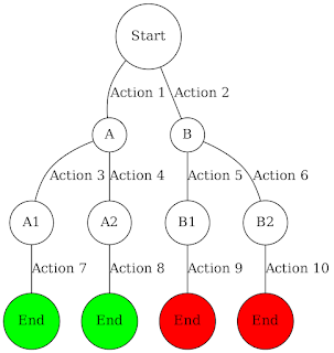
 A state space tree is a graphical representation of all possible states and transitions in a decision-making problem, such as an optimization or search problem. It's often used in algorithms that explore the set of all possible solutions to find an optimal solution, such as the branch and bound method for optimization problems, or backtracking algorithms for constraint satisfaction problems.   Components and characteristics of a state space tree:   1. Nodes:    - Each node represents a state of the problem .    - The root node represents the initial state before any decisions have been made.    - Intermediate nodes represent partial decisions or partial solutions.    - Leaf nodes (at the bottom of the tree) represent complete solutions or end states.   2. Edges/Branches:    - Edges connect nodes and represent transitions from one state to another due to a decision or action.    - Each edge often has an associated cost or value if it's an optimization probl

 Sample Assignment Problem State Space Tree The root node represents the starting point where no assignments have been made yet. Each branch from the root represents a possible job assignment for Worker 1 (denoted as x1). The second level represents possible assignments for Worker 2 (denoted as x2), given the job already assigned to Worker 1. In a full state space tree, this process would continue for Workers 3 and 4, each with their own level in the tree, until all workers are assigned jobs without conflict, resulting in a complete solution at the leaf nodes. Full state Space Tree Each path from the root to a leaf node represents a complete set of job assignments, one for each worker. There are 4! = 24 possible paths, each corresponding to a different way to assign all four jobs to the four workers without any overlaps. ​

 The assignment problem is a fundamental combinatorial optimization problem that involves assigning resources to tasks in the most efficient way. It's commonly formulated as a problem of finding a maximum-weight or minimum-cost matching in a weighted bipartite graph.  Components Here are its main components: Example 1. Resources and Tasks:    - In the assignment problem, there are typically two sets: a set of resources (such as workers, machines) and a set of tasks (such as jobs, processes). The goal is to assign each resource to exactly one task, and vice versa. 2. Cost Matrix:    - The problem is often represented using a cost matrix (or benefit matrix, in case of a maximization problem). This matrix provides the cost (or benefit) of assigning each resource to each task. For instance, in a cost matrix, the element at the i-th row and j-th column represents the cost of assigning the i-th resource to the j-th task. 3. Objective Function: 4. Constraints:    - Each resourc

 A Constraint Satisfaction Problem (CSP) is a type of problem in which the goal is to find a set of variable assignments that satisfy a given set of constraints. CSPs are commonly found in various fields like artificial intelligence, computer science, and operations research.  Components The key components of a CSP are:   1. Variables:      A set of variables that need to be assigned values. For example, in a scheduling problem, variables could be time slots for different tasks.   2. Domains:      Each variable has a domain, which is the set of possible values it can take. For instance, if the variable is "color of a shirt," the domain might be {red, blue, green}.   3. Constraints:      Constraints specify the conditions that the variables' values must collectively satisfy. They limit the combinations of values the variables can take. For example, a constraint in a scheduling problem could be that two particular tasks cannot occur at the same time.      Cons

  An optimization problem is a mathematical problem that involves finding the best solution from all feasible solutions.  Main Components It typically consists of three main components:   1. Objective Function:  This is a function that needs to be optimized (either maximized or minimized). It could represent various real world goals such as cost, profit, efficiency, utility, or distance. The objective function is defined in terms of decision variables, and the goal is to find the values of these variables that optimize the function.   2. Decision Variables:  These are the variables that the optimization algorithm adjusts to find the best solution. The values of these variables determine the behavior or configuration of the system being studied. For example, in a transportation problem, decision variables could represent the number of goods to be shipped from each source to each destination.   3. Constraints:  Constraints are conditions that the solution must satisfy. They limit t

  Space complexity analysis involves evaluating how much memory space an algorithm uses in terms of the size of the input. It's an important aspect of algorithm design, especially for memoryconstrained environments.     Performing Space Complexity Analysis   1. Identify Variables and Data Structures: Determine the variables, arrays, objects, and other data structures used in the algorithm and how their size changes with the input.   2. Account for Auxiliary Space: Consider additional memory used by the algorithm (apart from the input data) for variables, data structures, etc.   3. Consider Recursion Stack: In recursive algorithms, consider the maximum depth of the recursion stack.   4. Sum Up All Memory Uses: Add up the memory used by different components to estimate the total space requirement.   5. Express in Big O Notation: Represent the space complexity using Big O notation, focusing on how it scales with input size.     Types of Space Complexity   1. Constant S

    1. Constant Time (O(1)):  The execution time remains constant regardless of input size.  Occurrence: When the algorithm performs a fixed number of operations, regardless of the input size. Example: Accessing an element in an array by index, checking if a stack is empty.   2. Logarithmic Time (O(log n)):  The execution time grows logarithmically with the input size.  Occurrence: When the algorithm reduces the problem size by a factor (usually half) in each step. Example: Binary search in a sorted array, finding an item in a balanced binary search tree.   3. Linear Time (O(n)):  The execution time grows linearly with the input size.  Occurrence: When the algorithm must look at every element of the input once. Example: Finding the maximum element in an unsorted array, linear search.   4. Linearithmic Time (O(n log n)):  The execution time grows linearithmically with the input size. Occurrence: When the algorithm combines a logarithmic reduction of problem size with a linear scan. Exam

  Performing algorithm analysis involves evaluating the efficiency of an algorithm, primarily in terms of time complexity and space complexity. Time complexity refers to the amount of time an algorithm takes to complete as a function of the length of the input, while space complexity refers to the amount of memory space required by the algorithm.     Steps for Performing Algorithm Analysis   1. Identify the Basic Operation:  Determine the fundamental operation of the algorithm. This is usually the most frequent operation, like a comparison in a sorting algorithm. 2. Establish Input Size:  Define what constitutes the input size. For instance, in sorting, it's the number of elements to be sorted.   3. Count the Operations:  Analyze how the number of basic operations scales with the input size. This can be in the best, worst, and average cases.   4. Determine the Time Complexity:  Express how the total number of operations grows with the input size. This is often done using

 The Change Making Problem is a classic optimization problem where the goal is to make change for a specific amount using the fewest number of coins from a given set of denominations. When approaching this problem with a brute force method, it involves examining all possible combinations of coins that add up to the given amount and selecting the combination with the minimum number of coins.   Brute Force Solution for Change Making Problem   Problem Setup:  Given a set of coin denominations (e.g., `[1, 5, 10]`) and a total amount (e.g., `12`), find the minimum number of coins that make up that amount.   Brute Force Approach:     1. Generate All Combinations:  Produce all combinations of coins that sum up to the target amount. This usually requires recursion, where you explore each possible way to reach the amount using the given denominations.     2. Select Minimum Coin Combination:  For each combination that sums to the target amount, count the number of coins used. Keep trac

  A problem where a brute force approach is often considered the best or a very suitable method is the Traveling Salesman Problem (TSP) for very small datasets. The TSP involves finding the shortest possible route that visits a set of cities exactly once and returns to the origin city.   Why Brute Force is Suitable for TSP with Small Datasets: 1. Simplicity and Completeness:  For a very small number of cities, a brute force approach is simple to implement and guarantees finding the shortest possible route, as it checks every possible permutation of the cities. 2. Guaranteed Optimal Solution:  Since brute force explores every possible tour, it ensures that the best solution is not missed, which is crucial in problems where finding the absolute best solution is more important than the efficiency of the algorithm. 3. Small Dataset Manageability:  With a small number of cities (e.g., 5-10 cities), the number of permutations remains within a manageable limit, making the brute force